Activity 4 | Histogram Backprojection

Images are comprised of pixels with values that represent a certain color. Getting the histogram of these pixel values give us information on the spread of the image's color from say black '0' to white '1' like grayscale images. In the previous activity, the histogram of a grayscale image was used to enhance the image by thresholding such that the desired region is well separated from the background.

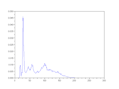
In this activity, image enhancement is once again performed by tweaking the cumulative distribution function or the normalized histogram of a grayscale image into functions like the linear, parabolic, and logarithmic functions. Let us examine the PDF and CDF of a sample grayscale image as shown in Figure 1.

Figure 1. Original image with PDF and CDF respectively.

Performing histogram backprojection on the image using a linear CDF shown in Figure 2, we get a new image, its PDF and CDF as shown in Figure 3. From the image, PDF and CDF of the new image we can see the presence of higher values making the image brighter and more even.

Figure 2. Linear CDF.

Figure 3. New image with PDF and linear CDF.

Performing histogram backprojection on the image using a parabolic CDF shown in Figure 4, we get another new image, its PDF and CDF as shown in Figure 5. Because of the shape of the parabolic CDF, the majority of the pixels have high values thus producing an image with the very bright areas that are not needed as seen in the new x-ray image making it saturated.

Figure 4. Parabolic CDF.

Figure 5. New image with PDF and parabolic CDF.

Now the human eye has a nonlinear response, specifically a logarithmic response so using a logarithmic CDF shown in Figure 6, we get a new image, its PDF and CDF as shown in Figure 7. Because of the logarithmic trend, the resulting image has high contrast than the linear CDF. The logarithmic response is repeated on another image as shown in Figure 8.

Figure 6. Logarithmic CDF.

Figure 7. Using a logarithmic CDF.

Figure 8. Simulation of human eye response using a logarithmic CDF with original image (left) and new image (right) using logarithmic CDF.

I give myself a grade of 9 for this activity since I was able to do the histogram back projection using different CDFs and was able to produce the PDFs and CDFs of the new images correctly.